Introduction
Breast cancer research is crucial for improving diagnosis and treatment outcomes, potentially saving millions of lives. Bioinformatics plays a vital role in this field by enabling the analysis of complex genetic data to uncover insights into cancer biology. In this project, titled “Advanced Breast Cancer Research and Multi-Class Detection Using RNA-Seq,” I aimed to apply RNA sequencing analysis techniques to identify gene expression patterns across different breast cancer subtypes (TNBC, Non-TNBC, HER2-positive) and healthy tissues. The goal was to develop and deploy a machine learning model to classify breast tissue samples based on their gene expression profiles.
Phase 1: Project Setup and Initial Data Handling
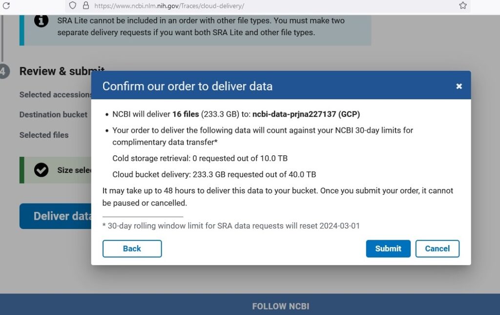
Step 1: Create a Cloud Storage Bucket The first step was to create a Cloud Storage bucket named ncbi-data-prjna227137 to store all my project data.
gsutil mb gs://ncbi-data-prjna227137Step 2: Data Collection Next, I collected data from the public NCBI dataset (GSE52194) and stored it in the Cloud Storage bucket. Using NCBI’s SRA Run Selector service, I downloaded patient metadata and FASTQ files directly to Cloud Storage by granting temporary Storage Object Admin access to NCBI’s service account. After completion, I received a confirmation email indicating the data was successfully delivered.
Phase 2: Data Preprocessing and Feature Selection
Step 3: Build and Upload a Container Image I built Docker containers for RNA sequence analysis. Below is the Dockerfile I used:
FROM continuumio/miniconda3
RUN apt-get update && apt-get install -y \
    procps \
    cutadapt \
    fastqc \
    rsem \
    bwa \
    samtools \
    bcftools
I built and ran the Docker image:
docker build -t my_rna_seq_image -f Dockerfile .
docker run -it --name my_rna_seq_container my_rna_seq_image /bin/bash
Due to dependency issues with trim-galore, I created a new conda environment with Python 3.9:
conda create -n new_env python=3.9
conda activate new_env
conda install -c bioconda trim-galore
Step 4: Downloading the Reference Genome and Annotation Files: For this project, I obtained the necessary reference genome and annotation files from Ensembl useing the following wget command. This ensured that I had the most up-to-date and accurate data for human genome analysis
wget -P /rna-seq-folder/ https://ftp.ensembl.org/pub/release-110/fasta/homo_sapiens/dna/Homo_sapiens.GRCh38.dna_sm.primary_assembly.fa.gz
wget -P /rna-seq-folder/ https://ftp.ensembl.org/pub/release-112/gtf/homo_sapiens/Homo_sapiens.GRCh38.110.gtf.gz
Unzip the downloaded files:
gunzip /rna-seq-folder/Homo_sapiens.GRCh38.dna_sm.primary_assembly.fa.gz
gunzip /rna-seq-folder/Homo_sapiens.GRCh38.110.gtf.gz
Step 5: Preparing the Reference for RSEM: With the reference genome and annotation files downloaded and unzipped, I executed the following command to prepare the reference:
rsem-prepare-reference --gtf /rna-seq-folder/Homo_sapiens.GRCh38.110.gtf --star /rna-seq-folder/Homo_sapiens.GRCh38.dna_sm.primary_assembly.fa /rna-seq-folder/ref/human_rsem_ref
Step 6: Automate Data Processing
I wrote a script to automate downloading, quality checking, and trimming RNA-Seq data:
bash
#!/bin/bash
start=1027171
end=1027190
for ((i=start; i<=end; i++))
do
    bucket_path="gs://ncbi-data-prjna227137/SRR$i/"
    gsutil -m cp "${bucket_path}*" .
    fastqc SRR${i}/*sequence.txt.gz
    trim_galore --quality 20 --fastqc --paired SRR${i}/*_1_sequence.txt.gz SRR${i}/*_2_sequence.txt.gz
    gsutil cp SRR${i}/*trimmed.fq.gz "${bucket_path}"
done
I made the script executable and ran it:
chmod +x process_rna_seq.sh
./process_rna_seq.sh
This phase involved setting up a robust framework for the project and ensuring the initial data handling processes were thorough and well-documented. The quality control, read alignment, and expression quantification steps laid a solid foundation for subsequent phases of the project.
Phase 3: Data Integration and Analysis
Step 7: Align and Estimate Expression with RSEM I ran RSEM to align reads and estimate gene and isoform expressions using the following script:
#!/bin/bash
cd /rna-seq-folder/fastq
for file in *_1_sequence.txt.gz; do
    base=$(basename $file _1_sequence.txt.gz)
    read1=${base}_1_sequence.txt.gz
    read2=${base}_2_sequence.txt.gz
    rsem-calculate-expression --paired-end --star --num-threads 16 \
        $read1 $read2 \
        /rna-seq-folder/ref/human_rsem_ref \
        /rna-seq-folder/results/${base}
done
I made the script executable and ran it:
chmod +x run_rsem.sh
./run_rsem.sh
Step 8: Convert RNA-Seq Output to CSV I converted the .results files to .csv format using the following script:
#!/bin/bash
for file in *.results; do
    newfile="${file%.results}.csv"
    awk 'BEGIN{FS="\t";OFS=","} {gsub(/ /, "\",\"", $2); print "\"" $1 "\",\"" $2 "\",\"" $3 "\",\"" $4 "\",\"" $5 "\",\"" $6 "\",\"" $7 "\""}' "$file" > "$newfile"
    echo "Converted $file to $newfile"
done
I made the script executable and ran it:
chmod +x convert_results_to_csv.sh
./convert_results_to_csv.sh
Step 9: Combining Data in Google Colab
After preparing the RNA-Seq output data, I needed to combine multiple CSV files laterally to create a matrix format suitable for DESeq2 analysis. Here’s how I did it:
Step 1: Set Up the Environment I ensured the pandas library was available for data manipulation:
Step 2: Upload Files to Google Colab In Colab, I uploaded the CSV files to the session storage using the sidebar.
Step 3: Import Pandas I imported pandas in the notebook:
!pip install pandas
import pandas as pd
import os
Step 10: Read and Combine Data Horizontally I wrote a script to read each CSV file and merge them horizontally based on the gene_id column:
# Initialize an empty DataFrame or the first DataFrame
key_df = None

# List all files and merge them horizontally
for filename in os.listdir('/content'):
    if filename.endswith('.csv'):
        # Read the CSV file
        data = pd.read_csv('/content/' + filename)

        # Extract the sample identifier from the filename
        sample_id = filename.replace('.csv', '')

        # Select and rename the necessary columns
        data = data[['gene_id', 'expected_count']].rename(columns={'expected_count': sample_id})

        if key_df is None:
            key_df = data
        else:
            # Merge while avoiding duplicate column names
            key_df = key_df.merge(data, on='gene_id', how='outer')

# Handle any missing values or discrepancies
key_df.fillna(0, inplace=True)
print(key_df.head())

# Save the merged DataFrame to a CSV file
output_file_path = '/content/merged_data.csv'
key_df.to_csv(output_file_path, index=False)

print(f"Merged data has been saved to {output_file_path}")
This project demonstrates the integration of RNA-Seq data analysis with cloud computing and machine learning to classify breast cancer subtypes. By following a structured approach, I overcame various challenges and successfully automated data processing and analysis workflows, showcasing the potential for scalable and efficient genomic research in the cloud.
Phase 4: Differential Expression Analysis
Step 11: Set Up DESeq2 in R Environment and Run DESeq2 Analysis
- I installed DESeq2 and other necessary packages, loaded the libraries, and set up the DESeq2 environment.
- I loaded the count data and created the metadata for the dataset. The metadata includes the condition for each sample (Normal, HER2, NonTNBC, TNBC).
- I then I created a DESeq2 dataset using the count data and metadata and ran the DESeq2 analysis to identify differentially expressed genes
# Install and load necessary packages
install.packages("pheatmap")
if (!requireNamespace("BiocManager", quietly = TRUE))
    install.packages("BiocManager")
BiocManager::install("biomaRt")
BiocManager::install("DESeq2")
BiocManager::install("clusterProfiler")
BiocManager::install("org.Hs.eg.db")
BiocManager::install("ReactomePA")
library(pheatmap)
library(biomaRt)
library(DESeq2)
library(clusterProfiler)
library(org.Hs.eg.db)
library(ReactomePA)

# Load count data (replace the file path with your actual path)
count_data <- read.csv("/content/count_data.csv", row.names = 1)

# Create metadata for the full dataset
metadata <- data.frame(
  row.names = colnames(count_data),
  condition = c(rep("Normal", 3), rep("HER2", 5), rep("NonTNBC", 6), rep("TNBC", 5))
)

# Convert non-integer values to integers by rounding
count_data <- round(count_data)
# Create DESeq2 dataset for the full dataset
dds <- DESeqDataSetFromMatrix(countData = count_data, colData = metadata, design = ~ condition)

# Pre-filtering (Optional) Remove rows with low counts to improve computation
dds <- dds[rowSums(counts(dds)) > 1, ]

# Normalize the data and run DESeq2 analysis
dds <- DESeq(dds)

# Extract normalized counts
normalized_counts <- counts(dds, normalized = TRUE)
Step 12: Differential Expression Analysis
- I performed differential expression analysis for each condition compared to Normal.
- I defined significance thresholds and extracted significant results (adjusted p-value < 0.05, log2FoldChange > 1).
- I identified the top differentially expressed genes for each comparison.
# Perform differential expression analysis for each condition vs Normal
res_her2_vs_normal <- results(dds, contrast = c("condition", "HER2", "Normal"))
res_non_tnbc_vs_normal <- results(dds, contrast = c("condition", "NonTNBC", "Normal"))
res_tnbc_vs_normal <- results(dds, contrast = c("condition", "TNBC", "Normal"))

# Define significance thresholds for heatmap, Volcano, & MA plot
padj_threshold <- 0.05
log2fc_threshold <- 1

# Extract significant results (adjusted p-value < 0.05, log2FoldChange > 1)
sig_HER2_vs_Normal <- subset(res_her2_vs_normal, padj < padj_threshold & abs(log2FoldChange) > log2fc_threshold)
sig_NonTNBC_vs_Normal <- subset(res_non_tnbc_vs_normal, padj < padj_threshold & abs(log2FoldChange) > log2fc_threshold)
sig_TNBC_vs_Normal <- subset(res_tnbc_vs_normal, padj < padj_threshold & abs(log2FoldChange) > log2fc_threshold)

# Top genes for each comparison
top_genes_HER2 <- rownames(head(sig_HER2_vs_Normal[order(sig_HER2_vs_Normal$padj), ], 50))
top_genes_NonTNBC <- rownames(head(sig_NonTNBC_vs_Normal[order(sig_NonTNBC_vs_Normal$padj), ], 50))
top_genes_TNBC <- rownames(head(sig_TNBC_vs_Normal[order(sig_TNBC_vs_Normal$padj), ], 50))
Step 12: Convert Ensembl IDs to Gene Symbols and Entrez IDs
- I converted Ensembl IDs to gene symbols and Entrez IDs using the biomaRt package.
# Convert Ensembl IDs to Gene Symbols and Entrez IDs
mart <- useDataset("hsapiens_gene_ensembl", useMart("ensembl"))
convert_ids <- function(ensembl_ids) {
    ids <- getBM(filters = "ensembl_gene_id",
                 attributes = c("ensembl_gene_id", "hgnc_symbol", "entrezgene_id"),
                 values = ensembl_ids,
                 mart = mart)
    ids <- ids[match(ensembl_ids, ids$ensembl_gene_id), ]  # Ensure the order matches the input
    ids$hgnc_symbol[is.na(ids$hgnc_symbol)] <- ids$ensembl_gene_id[is.na(ids$hgnc_symbol)]
    return(ids)
}

# Convert top genes to gene symbols and Entrez IDs
top_genes_HER2_ids <- convert_ids(top_genes_HER2)
top_genes_NonTNBC_ids <- convert_ids(top_genes_NonTNBC)
top_genes_TNBC_ids <- convert_ids(top_genes_TNBC)
Step 13: Save Significant Results
- I added gene symbols to significant results and saved them to CSV files.
# Add gene symbols to significant results
sig_HER2_vs_Normal$gene_symbol <- convert_ids(rownames(sig_HER2_vs_Normal))$hgnc_symbol
sig_NonTNBC_vs_Normal$gene_symbol <- convert_ids(rownames(sig_NonTNBC_vs_Normal))$hgnc_symbol
sig_TNBC_vs_Normal$gene_symbol <- convert_ids(rownames(sig_TNBC_vs_Normal))$hgnc_symbol

# Reorder columns to have gene_symbol first
sig_HER2_vs_Normal <- sig_HER2_vs_Normal[, c("gene_symbol", names(sig_HER2_vs_Normal)[-ncol(sig_HER2_vs_Normal)])]
sig_NonTNBC_vs_Normal <- sig_NonTNBC_vs_Normal[, c("gene_symbol", names(sig_NonTNBC_vs_Normal)[-ncol(sig_NonTNBC_vs_Normal)])]
sig_TNBC_vs_Normal <- sig_TNBC_vs_Normal[, c("gene_symbol", names(sig_TNBC_vs_Normal)[-ncol(sig_TNBC_vs_Normal)])]

# Sort significant results by adjusted p-value
sig_HER2_vs_Normal <- sig_HER2_vs_Normal[order(sig_HER2_vs_Normal$padj), ]
sig_NonTNBC_vs_Normal <- sig_NonTNBC_vs_Normal[order(sig_NonTNBC_vs_Normal$padj), ]
sig_TNBC_vs_Normal <- sig_TNBC_vs_Normal[order(sig_TNBC_vs_Normal$padj), ]

# Save significant results to CSV files with gene symbols as rownames
write.csv(sig_HER2_vs_Normal, "sig_her2_vs_normal.csv", row.names = FALSE)
write.csv(sig_NonTNBC_vs_Normal, "sig_non_tnbc_vs_normal.csv", row.names = FALSE)
write.csv(sig_TNBC_vs_Normal, "sig_tnbc_vs_normal.csv", row.names = FALSE)
| gene_symbol.hgnc | log2FoldChange | pvalue | padj |
|---|---|---|---|
| RPPH1 | 13.120665 | 4.82e-125 | 1.70e-120 |
| RN7SL1 | 10.489661 | 5.37e-119 | 9.46e-115 |
| RMRP | 11.149963 | 2.34e-109 | 2.74e-105 |
| SCARNA7 | 9.912687 | 1.50e-87 | 1.32e-83 |
| RN7SL2 | 9.188408 | 5.38e-85 | 3.79e-81 |
| SNORD3A | 11.934661 | 4.36e-82 | 2.56e-78 |
| RNU1-27P | 14.122484 | 5.41e-80 | 1.90e-76 |
| RNU1-2 | 14.122484 | 5.41e-80 | 1.90e-76 |
| RNU1-4 | 14.122484 | 5.41e-80 | 1.90e-76 |
| RNVU1-29 | 14.122484 | 5.41e-80 | 1.90e-76 |
| 10.763495 | 1.20e-76 | 3.83e-73 | |
| SNORA73B | 12.135523 | 3.70e-76 | 1.08e-72 |
| SCARNA2 | 9.716538 | 9.39e-75 | 2.54e-71 |
| RN7SK | 10.376260 | 2.32e-71 | 5.84e-68 |
| PPP1R15A | -7.007382 | 9.80e-66 | 2.30e-62 |
| MAFF | -7.113582 | 8.15e-64 | 1.79e-60 |
| 13.666196 | 9.85e-53 | 2.04e-49 | |
| H1-4 | 8.177815 | 4.96e-51 | 9.71e-48 |
| SKP2 | 4.212157 | 1.93e-50 | 3.57e-47 |
| GADD45A | -6.132037 | 3.91e-49 | 6.88e-46 |
| gene_symbol.hgnc | log2FoldChange | pvalue | padj |
|---|---|---|---|
| RPPH1 | 13.337359 | 1.57e-136 | 5.37e-132 |
| RN7SL1 | 10.061270 | 8.76e-117 | 1.50e-112 |
| RMRP | 10.242729 | 2.14e-98 | 2.45e-94 |
| RN7SL2 | 9.581003 | 2.94e-98 | 2.52e-94 |
| SCARNA2 | 10.275627 | 1.04e-87 | 7.10e-84 |
| SCARNA7 | 9.645241 | 4.28e-86 | 2.44e-82 |
| SNORA73B | 11.588326 | 4.75e-72 | 2.33e-68 |
| SNORD3A | 10.433383 | 4.33e-67 | 1.86e-63 |
| MAFF | -6.885642 | 4.42e-65 | 1.68e-61 |
| PCBP1 | -3.491532 | 9.62e-65 | 3.30e-61 |
| RN7SK | 9.428783 | 4.64e-63 | 1.44e-59 |
| PPP1R15A | -6.360018 | 1.22e-58 | 3.29e-55 |
| 9.102245 | 1.25e-58 | 3.29e-55 | |
| RPL36A | -4.799584 | 5.54e-56 | 1.36e-52 |
| RNU1-27P | 11.463050 | 1.97e-55 | 3.75e-52 |
| RNU1-2 | 11.463050 | 1.97e-55 | 3.75e-52 |
| RNU1-4 | 11.463050 | 1.97e-55 | 3.75e-52 |
| RNVU1-29 | 11.463050 | 1.97e-55 | 3.75e-52 |
| UBC | -5.645960 | 4.05e-55 | 7.31e-52 |
| TIPARP | -4.146750 | 1.83e-52 | 3.13e-49 |
| gene_symbol.hgnc | log2FoldChange | pvalue | padj |
|---|---|---|---|
| RPPH1 | 13.056331 | 7.70e-124 | 2.86e-119 |
| RN7SL1 | 9.358069 | 4.19e-95 | 7.77e-91 |
| SCARNA7 | 9.500841 | 1.45e-80 | 1.79e-76 |
| SCARNA2 | 10.044002 | 9.35e-80 | 8.67e-76 |
| RMRP | 9.311857 | 7.55e-77 | 5.60e-73 |
| RN7SL2 | 8.699062 | 2.22e-76 | 1.38e-72 |
| TIPARP | -5.004191 | 2.15e-69 | 1.14e-65 |
| PCBP1 | -3.575154 | 3.51e-63 | 1.63e-59 |
| 9.193054 | 2.10e-56 | 8.65e-53 | |
| H4C5 | 8.826695 | 3.26e-55 | 1.21e-51 |
| ZFP36 | -8.188346 | 1.23e-51 | 4.16e-48 |
| SNORA73B | 9.879655 | 4.59e-51 | 1.42e-47 |
| UBC | -5.592576 | 8.10e-51 | 2.31e-47 |
| RN7SK | 8.658679 | 3.04e-50 | 8.05e-47 |
| MAFF | -6.170424 | 1.49e-49 | 3.68e-46 |
| RPL36A | -4.607554 | 2.49e-48 | 5.76e-45 |
| PCBP2 | -3.097582 | 3.56e-48 | 7.78e-45 |
| NXF1 | -3.854211 | 5.80e-47 | 1.20e-43 |
| PPP1R15A | -5.834175 | 1.26e-46 | 2.47e-43 |
| ZC3H12A | -4.988088 | 1.72e-46 | 3.19e-43 |
Step 14: Create PCA and Heatmaps
- Principal Component Analysis (PCA) was performed to visualize the variance in the dataset.
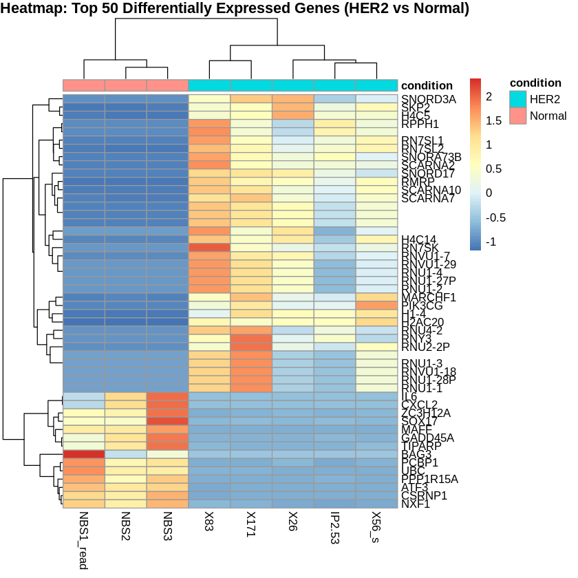
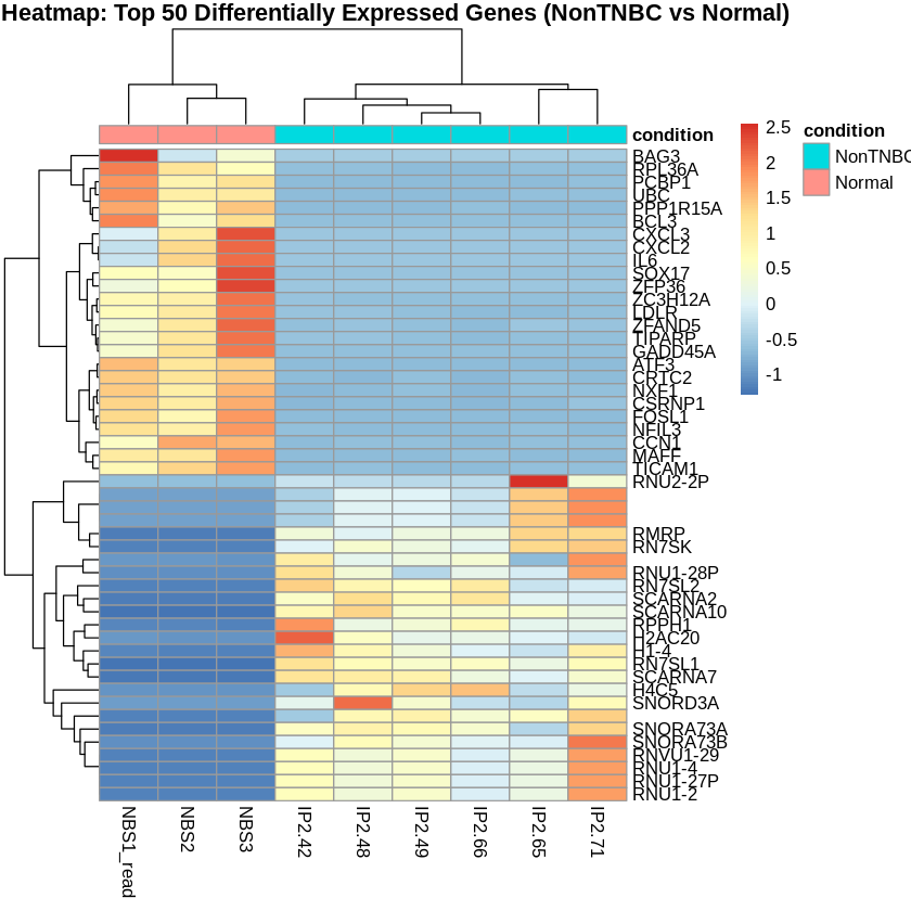
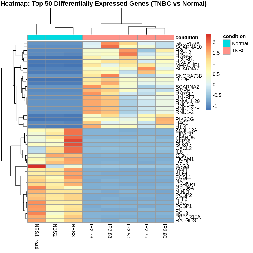
- I created heatmaps to visualize the top 50 differentially expressed genes for each comparison.
# Extract relevant samples for each comparison
her2_samples <- c("NBS1_read", "NBS2", "NBS3", "X26", "IP2.53", "X56_s", "X83", "X171")
nontnbc_samples <- c("NBS1_read", "NBS2", "NBS3", "IP2.42", "IP2.48", "IP2.49", "IP2.65", "IP2.66", "IP2.71")
tnbc_samples <- c("NBS1_read", "NBS2", "NBS3", "IP2.50", "IP2.76", "IP2.78", "IP2.83", "IP2.90")

# Filter the normalized counts for top genes and relevant samples
normalized_counts_HER2 <- normalized_counts[top_genes_HER2, her2_samples]
normalized_counts_NonTNBC <- normalized_counts[top_genes_NonTNBC, nontnbc_samples]
normalized_counts_TNBC <- normalized_counts[top_genes_TNBC, tnbc_samples]

# Rename rows to gene symbols
rownames(normalized_counts_HER2) <- top_genes_HER2_ids$hgnc_symbol
rownames(normalized_counts_NonTNBC) <- top_genes_NonTNBC_ids$hgnc_symbol
rownames(normalized_counts_TNBC) <- top_genes_TNBC_ids$hgnc_symbol

# Scale the counts
scaled_counts_HER2 <- t(scale(t(normalized_counts_HER2)))
scaled_counts_NonTNBC <- t(scale(t(normalized_counts_NonTNBC)))
scaled_counts_TNBC <- t(scale(t(normalized_counts_TNBC)))

# Create metadata for relevant samples
metadata_HER2 <- metadata[her2_samples, , drop=FALSE]
metadata_NonTNBC <- metadata[nontnbc_samples, , drop=FALSE]
metadata_TNBC <- metadata[tnbc_samples, , drop=FALSE]

# Create heatmaps
pheatmap(scaled_counts_HER2, cluster_rows = TRUE, cluster_cols = TRUE,
         show_rownames = TRUE, show_colnames = TRUE,
         annotation_col = metadata_HER2,
         main = "Heatmap: Top 50 Differentially Expressed Genes (HER2 vs Normal)")

pheatmap(scaled_counts_NonTNBC, cluster_rows = TRUE, cluster_cols = TRUE,
         show_rownames = TRUE, show_colnames = TRUE,
         annotation_col = metadata_NonTNBC,
         main = "Heatmap: Top 50 Differentially Expressed Genes (NonTNBC vs Normal)")

pheatmap(scaled_counts_TNBC, cluster_rows = TRUE, cluster_cols = TRUE,
         show_rownames = TRUE, show_colnames = TRUE,
         annotation_col = metadata_TNBC,
         main = "Heatmap: Top 50 Differentially Expressed Genes (TNBC vs Normal)")

vsd <- vst(dds, blind = FALSE)
pcaData <- plotPCA(vsd, intgroup = "condition", returnData = TRUE)
percentVar <- round(100 * attr(pcaData, "percentVar"))

ggplot(pcaData, aes(PC1, PC2, color = condition)) +
  geom_point(size = 3) +
  xlab(paste0("PC1: ", percentVar[1], "% variance")) +
  ylab(paste0("PC2: ", percentVar[2], "% variance")) +
  theme_minimal() +
  ggtitle("PCA Plot of Normalized Counts")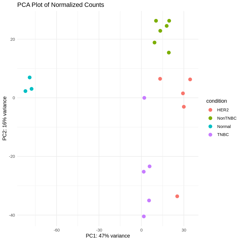
Step 15: MA Plot and Volcano Plot
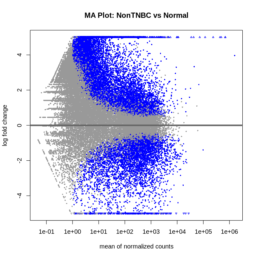
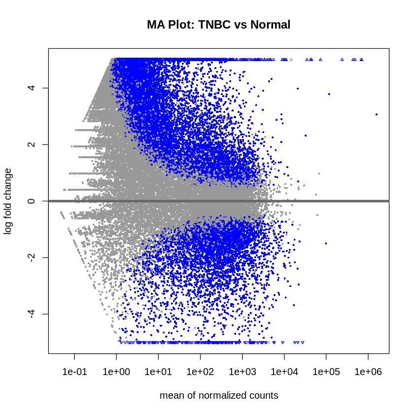
- MA plots were created to visualize the log2 fold changes versus the mean of normalized counts.
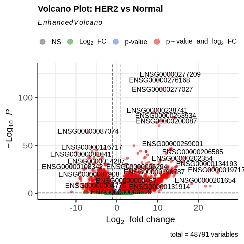
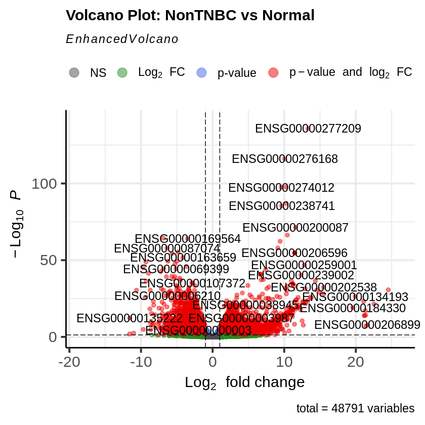
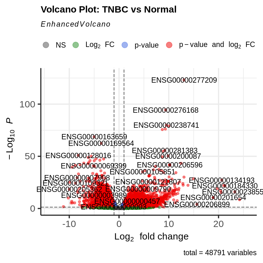
- Volcano plots were generated to visualize the significance versus fold-change of genes.
plotMA(res_her2_vs_normal, main = "MA Plot: HER2 vs Normal", ylim = c(-5, 5))
plotMA(res_non_tnbc_vs_normal, main = "MA Plot: NonTNBC vs Normal", ylim = c(-5, 5))
plotMA(res_tnbc_vs_normal, main = "MA Plot: TNBC vs Normal", ylim = c(-5, 5))

EnhancedVolcano(res_her2_vs_normal,
                lab = rownames(res_her2_vs_normal),
                x = 'log2FoldChange',
                y = 'pvalue',
                title = 'Volcano Plot: HER2 vs Normal',
                pCutoff = padj_threshold,
                FCcutoff = log2fc_threshold)

EnhancedVolcano(res_non_tnbc_vs_normal,
                lab = rownames(res_non_tnbc_vs_normal),
                x = 'log2FoldChange',
                y = 'pvalue',
                title = 'Volcano Plot: NonTNBC vs Normal',
                pCutoff = padj_threshold,
                FCcutoff = log2fc_threshold)

EnhancedVolcano(res_tnbc_vs_normal,
                lab = rownames(res_tnbc_vs_normal),
                x = 'log2FoldChange',
                y = 'pvalue',
                title = 'Volcano Plot: TNBC vs Normal',
                pCutoff = padj_threshold,
                FCcutoff = log2fc_threshold)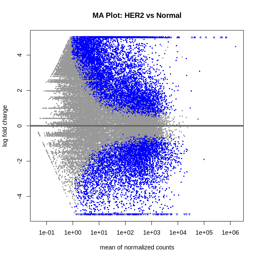
Phase 5: Enrichment Analysis
Step 16: Gene Ontology (GO), KEGG Pathway Enrichment, and Reactome Pathway Enrichment Analysis
- I performed GO enrichment analysis, KEGG pathway enrichment analysis, and Reactome Pathway Enrichment Analysis using the significant genes.
# Extract Entrez IDs for enrichment analysis
entrez_ids_her2_vs_normal <- na.omit(convert_ids(rownames(sig_HER2_vs_Normal))$entrezgene_id)
entrez_ids_non_tnbc_vs_normal <- na.omit(convert_ids(rownames(sig_NonTNBC_vs_Normal))$entrezgene_id)
entrez_ids_tnbc_vs_normal <- na.omit(convert_ids(rownames(sig_TNBC_vs_Normal))$entrezgene_id)

# Perform GO enrichment analysis
ego_her2_vs_normal <- enrichGO(gene          = entrez_ids_her2_vs_normal,
                               OrgDb         = org.Hs.eg.db,
                               keyType       = "ENTREZID",
                               ont           = "ALL",
                               pAdjustMethod = "BH",
                               pvalueCutoff  = 0.05,
                               qvalueCutoff  = 0.05)

ego_non_tnbc_vs_normal <- enrichGO(gene          = entrez_ids_non_tnbc_vs_normal,
                                   OrgDb         = org.Hs.eg.db,
                                   keyType       = "ENTREZID",
                                   ont           = "ALL",
                                   pAdjustMethod = "BH",
                                   pvalueCutoff  = 0.05,
                                   qvalueCutoff  = 0.05)

ego_tnbc_vs_normal <- enrichGO(gene          = entrez_ids_tnbc_vs_normal,
                               OrgDb         = org.Hs.eg.db,
                               keyType       = "ENTREZID",
                               ont           = "ALL",
                               pAdjustMethod = "BH",
                               pvalueCutoff  = 0.05,
                               qvalueCutoff  = 0.05)

# Save GO enrichment results to CSV files
write.csv(as.data.frame(ego_her2_vs_normal), "go_enrichment_her2_vs_normal.csv")
write.csv(as.data.frame(ego_non_tnbc_vs_normal), "go_enrichment_non_tnbc_vs_normal.csv")
write.csv(as.data.frame(ego_tnbc_vs_normal), "go_enrichment_tnbc_vs_normal.csv")

# Perform KEGG pathway enrichment analysis
ekegg_her2_vs_normal <- enrichKEGG(gene         = entrez_ids_her2_vs_normal,
                                   organism     = "hsa",
                                   pvalueCutoff = 0.05)

ekegg_non_tnbc_vs_normal <- enrichKEGG(gene         = entrez_ids_non_tnbc_vs_normal,
                                       organism     = "hsa",
                                       pvalueCutoff = 0.05)

ekegg_tnbc_vs_normal <- enrichKEGG(gene         = entrez_ids_tnbc_vs_normal,
                                   organism     = "hsa",
                                   pvalueCutoff = 0.05)

# Save KEGG enrichment results to CSV files
write.csv(as.data.frame(ekegg_her2_vs_normal), "kegg_enrichment_her2_vs_normal.csv")
write.csv(as.data.frame(ekegg_non_tnbc_vs_normal), "kegg_enrichment_non_tnbc_vs_normal.csv")
write.csv(as.data.frame(ekegg_tnbc_vs_normal), "kegg_enrichment_tnbc_vs_normal.csv")

# Perform Reactome Pathway enrichment analysis
reactome_her2_vs_normal <- enrichPathway(gene          = entrez_ids_her2_vs_normal,
                                         organism      = "human",
                                         pvalueCutoff  = 0.05,
                                         pAdjustMethod = "BH")

reactome_non_tnbc_vs_normal <- enrichPathway(gene          = entrez_ids_non_tnbc_vs_normal,
                                             organism      = "human",
                                             pvalueCutoff  = 0.05,
                                             pAdjustMethod = "BH")

reactome_tnbc_vs_normal <- enrichPathway(gene          = entrez_ids_tnbc_vs_normal,
                                         organism      = "human",
                                         pvalueCutoff  = 0.05,
                                         pAdjustMethod = "BH")

# Save Reactome enrichment results to CSV files
write.csv(as.data.frame(reactome_her2_vs_normal), "reactome_enrichment_her2_vs_normal.csv")
write.csv(as.data.frame(reactome_non_tnbc_vs_normal), "reactome_enrichment_non_tnbc_vs_normal.csv")
write.csv(as.data.frame(reactome_tnbc_vs_normal), "reactome_enrichment_tnbc_vs_normal.csv")