Machine Learning for Breast Cancer Subtype Classification Using RNA-Seq Data

Introduction

Breast cancer subtyping is crucial for personalizing treatment and improving patient outcomes. In this project, I applied machine learning techniques to RNA-seq gene expression data to classify breast cancer subtypes (Normal, HER2-positive, TNBC, Non-TNBC). By combining dimensionality reduction and machine learning, I aimed to develop an accurate and scalable classification model.

In the earlier phases of this project, I processed RNA-seq data to generate gene expression counts, performed quality control, and prepared the data for analysis. Now, in this phase, I explore how machine learning techniques can be used to classify breast cancer subtypes—Normal, HER2-positive, TNBC, and Non-TNBC—using the processed gene expression data.

Data Preparation: Transposing and Merging the DataFrames

To facilitate analysis, the gene expression data (filtered_count_data) was transposed, converting rows to columns so that each sample becomes a column and each gene becomes a row. After transposing, the first row was set as the new header, and unnecessary indices were dropped.

Next, I merged this transposed data with the sample conditions from col_data, ensuring each sample in the gene expression data was associated with its corresponding condition (e.g., Normal, HER2-positive, TNBC). Finally, I concatenated the Conditions column back to the merged dataset for analysis.

# Transpose the filtered_count_data dataframe
filtered_count_data_transposed = filtered_count_data.T
filtered_count_data_transposed.reset_index(inplace=True)

# Set the first row as the new header
filtered_count_data_transposed.columns = filtered_count_data_transposed.iloc[0]
filtered_count_data_transposed = filtered_count_data_transposed.drop(filtered_count_data_transposed.index[0])

# Extract 'Conditions' column from col_data
conditions = col_data[['Conditions']]

# Merge transposed gene data with sample information, keeping 'gene_id' for reference
merged_df = pd.merge(col_data.drop(columns=['Conditions']), 
                     filtered_count_data_transposed, 
                     left_on='Sample', 
                     right_on='gene_id', 
                     how='right')

# Append 'Conditions' column back to the merged dataframe
merged_df_final = pd.concat([merged_df, conditions], axis=1)

Step 17: Dimensionality Reduction Using PCA

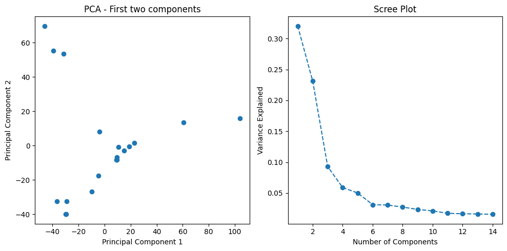
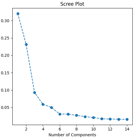
To manage the complexity of gene expression data, I first applied Principal Component Analysis (PCA). This technique reduced the high-dimensional data (thousands of genes) to a more manageable number of principal components that retain 95% of the data’s variance. This dimensionality reduction is essential for training machine learning models more efficiently and avoiding overfitting.

from sklearn.decomposition import PCA
from sklearn.preprocessing import StandardScaler

# Standardize the data
scaler = StandardScaler()
scaled_data = scaler.fit_transform(data.drop(columns=['gene_id', 'Conditions']))

# Apply PCA, retaining 95% of variance
pca = PCA(n_components=0.95)
principal_components = pca.fit_transform(scaled_data)

# Output number of components and explained variance
num_components = pca.n_components_
explained_variance = pca.explained_variance_ratio_

print(f"Number of components: {num_components}")
print(f"Explained variance: {explained_variance}")

I visualized the results of the PCA by plotting the first two principal components, which reveal how well different breast cancer subtypes are separated in the reduced feature space.

import matplotlib.pyplot as plt

# Scatter plot of first two components
plt.scatter(principal_components[:, 0], principal_components[:, 1], c=data['Conditions'].astype('category').cat.codes)
plt.title('PCA: First Two Components')
plt.xlabel('Principal Component 1')
plt.ylabel('Principal Component 2')
plt.show()

Step 18: Training Machine Learning Models

With the reduced dataset from PCA, I trained several machine learning classifiers to predict the breast cancer subtype based on gene expression profiles. The classifiers used include:

• Support Vector Machine (SVM)
• Random Forest
• Gradient Boosting
• K-Nearest Neighbors (KNN)
• Logistic Regression

Each model was trained using 5-fold cross-validation to ensure reliable performance estimates.

from sklearn.svm import SVC
from sklearn.model_selection import cross_val_score

# Define PCA-reduced features and labels
X = principal_components
y = data['Conditions'].values

# Train SVM model and perform cross-validation
svm_model = SVC(kernel='linear', C=1)
cross_val_scores = cross_val_score(svm_model, X, y, cv=5)

print(f"Mean cross-validation accuracy (SVM): {cross_val_scores.mean():.2f}")

Step 19: Comparing Model Performance

I compared the performance of various models by measuring their mean cross-validation accuracy. Here are the results:

from sklearn.ensemble import RandomForestClassifier, GradientBoostingClassifier
from sklearn.neighbors import KNeighborsClassifier
from sklearn.linear_model import LogisticRegression

# Initialize other models for comparison
classifiers = {
    "Random Forest": RandomForestClassifier(n_estimators=100),
    "Gradient Boosting": GradientBoostingClassifier(n_estimators=100),
    "K-Nearest Neighbors": KNeighborsClassifier(n_neighbors=3),
    "Logistic Regression": LogisticRegression(max_iter=1000)
}

# Evaluate each classifier using cross-validation
for name, clf in classifiers.items():
    scores = cross_val_score(clf, X, y, cv=5)
    print(f"{name}: Mean cross-validation accuracy = {scores.mean():.2f}")

Results:

Support Vector Machine (SVM) with a linear kernel achieved the highest accuracy of 88.33%.Random Forest, Gradient Boosting, and K-Nearest Neighbors (KNN) all achieved an accuracy of 80%.Logistic Regression also performed well with an accuracy of 88%, similar to SVM.

The SVM model performed best, highlighting its suitability for this RNA-seq classification task.